


 |
Services Offered this Issue
> The Appraiser Coach |
Editor’s Note: This story can be found in the new print edition of Working RE (just mailed). Am I a Working RE Subscriber? OREP E&O insureds enjoy a free subscription.
How Much Value Does That Extra Bedroom Add? (Understanding Regression)
By Dr. Keying Ye
In the simplest terms, real estate appraisers evaluate the fair market value of a property — one number that aggregates the value of a wide array of the property’s features, both quantitative (number of bedrooms and bathrooms, square footage, lot size, number of garages, etc.) and qualitative (views, street scene, location, etc.). Right?
One way to approximate this value is using the regression method, which is a data analysis tool for studying the relationship between a dependent variable (in this case, property value) and feature predictors (such as number of bathrooms or gross living area). This article aims to show how regression can increase appraisal accuracy by focusing on the two most common types: Simple vs. Multiple Linear Regression.
Tackling Simple Linear Regression
Simple linear regression (SLR) is a straightforward regression approach using only one predictor and one dependent variable. For example, if we believe that we can use living area as the sole predictor to estimate a property’s value and that the association between living area and the value of a property is linearly related, then we could use a simple linear regression to estimate the value.
A predictive structure of SLR can be expressed as prediction = m + b * feature.
In this case, feature is the independent variable and prediction is the response variable (think back to y = m + bx from high school algebra). Here “m” and “b” are the “slope” and “intercept,” respectively, of a graph made from this equation. The intercept is where the prediction would be if the feature is zero (if the subject property doesn’t have a garage for example). The slope is the increase or decrease in the property value for each unit change in the feature (e.g. how much the property’s value changes for every square foot added or subtracted).
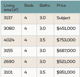
Consider the following example. We want to forecast the value of a singlefamily residence (SFR) and we know its basic information such as living area, number of beds, and number of baths. Using HouseCanary’s pre-computed comps analysis, we identify the five most similar properties sold within the last six months, as shown in the table below.
(story continues below)
(story continues)
The similarity is determined by property types (SFR or others), property features, and the geographical distances between those properties and the subject property. Since each property has the same number of bedrooms, this feature has no impact on the price among these properties other than as a fixed constant. The price variation, however, is clearly associated with living area and the number of baths.
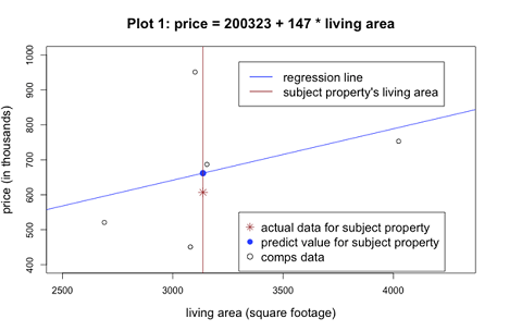
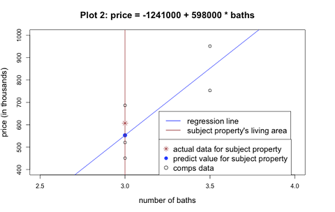
The figures below show the relationship between the property prices and either the living area or the number of baths of each of the properties (See plots 1 and 2). In each graph, the point where the vertical brown line touches the horizontal axis shows the subject property’s value for the feature in question (3,137 for living area and 3.0 for bathrooms). The blue line is the one-predictor linear regression line, which shows the predictive relationship between the property price and the appropriate feature.
(story continues below)
(story continues)
In plot 1, for example, the forecasting relationship between price and living area is expressed as: price =200,323 + 147 * living area. For the subject property, which measures 3,137 square feet, this means its predicted price is $661,462: $661,462 = ($200,323 + $147 * 3137) This is shown as the solid blue dot in the plot 1 graph. The “slope” of the regression line, 147, measures the unit price value, i.e., the price adjustment for each additional square-foot (plot 1). However, if we use number of bathrooms as our predictor instead, the target property’s predicted price is $553,000 (-$1,241,000 + $598,000 * 3.0 = $553,000). This discrepancy in predicted price ($661,462 and $553,000) is common when using simple linear regression formulas for different features of the same property (see plot 2 graph above).
The actual price for the target property is $607,000, which is shown as a brown star in each graph. Consequently, the errors for both estimates are nearly identical, albeit in the opposite direction, whether expressed in raw dollars ($607,000 – $661,462 = -$54,462 and $607,000 – $553,000 = $54,000, respectively) or as a percentage (-$54,462/$607,000 = – 9 percent and $54,000/$607,000 = 9 percent, respectively).
Going Further with Multiple Linear Regression
Using simple linear regression, an appraiser can use the most important predictor of a property’s value to make his/her appraisal analysis (or even use SLR analysis on multiple features to get multiple reference points. But what if the most important predictor isn’t clear? What if, for example, all of the three bedroom units in a given analysis have a different number of bathrooms, varying gross living areas, or only a couple of them have pools? By using multiple linear regression (MLR) appraisers can compare the effect that multiple predictors have on a property value with a single calculation.
A predictive structure of MLR can be expressed as:
prediction = m + b1 * feature 1 + b2 * feature 2 + b3 * feature 3+ …
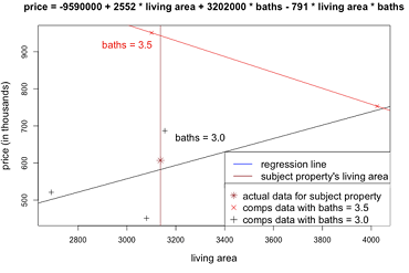
For example, with the data above, we can regress price by both living area and number of bathrooms: price = -$1,309,770 – $125 * living area + $744,918 * baths.
If we plug in the target property’s feature values, the predicted price is $532,859, which yields an error of $74,141 or 12%. The error of this prediction is worse than those errors considered in SLRs, but don’t worry, there is an explanation in the data (and a solution that follows!).
First, we must consider the relationships between the predictors themselves and understand what information the letters in the equation above convey, which is not as straightforward in this case as it was when using SLR. For instance, the coefficient -$125 for the living area says that, for a fixed number of baths, increasing living area by one square foot actually decreases the property price by $125 — which seems unnatural! However, if we look at the table above, we can see that for 3.5 bathrooms, there areonly two properties. The one with 3,101 square feet is actually more expensive ($951,000) than the property with 4,024 square feet. For the three properties with 3.0 bathrooms, the living areas (2690, 3080, 3155) don’t correlate exactly with the prices ($521,000, $451,000, $687,000) either.
(story continues below)

(story continues)
This means that, in our data, we have a different linear relationship between the response price and the predictor living area for the properties with a different number of bathrooms. Thus, in the next graph below, the black line (the regression line with baths = 3.0) and the red line (the regression line with baths = 3.5) actually show opposite trends. In such a case, both predictors are not purely additive against the price—an increase of onedoes not immediately imply an increase in the price. The remedy to this is to add another term, living area * number of baths, which represents the interaction of the predictors.
(story continues below)
(story continues)
For our data, the predictive relation would be expressed as:
price = -$9,590,000 + $2,552 * living area + 3,202,000 *baths – 791
* living area * baths
This yields a target property prediction of $577,523, which has an error of $29,477 ($607,000 – $577,523 = $29,477) and a relative error of 5 percent, which is the best fit so far!
When to Use Simple vs. Multiple Linear Regression
When appraising a property or determining the value of a particular feature, appraisers can use regression analysis to derive the most accurate price adjustments by taking into account the effect of multiple features on a property’s value. New industry regulations requiring data-driven justification for appraisal decisions may make regression analysis even more necessary for appraisers in the near future.
Keep in mind that it may not always be possible to use a multiple linear regression analysis. If, for example, there isn’t a varied array of data points available for a property and its comparables, there might not be enough information to conduct an MLR analysis. But, when there is enough available data to perform an MLR analysis, it often produces the most accurate results. Remember that there are times when an MLR analysis will require an additional term that represents the interaction of the predictors to be most accurate, such as in the example above. While regression analysis clearly doesn’t replace an appraiser’s expertise — it can be a valuable complement to it.
We hope you will find these insights useful for your appraisals.
> CE Online – 7 Hours (approved in 40 states)
How To Support and Prove Your Adjustments
Presented by: Richard Hagar, SRA
Must-know business practices for all appraisers working today. Ensure proper support for your adjustments. Making defensible adjustments is the first step in becoming a “Tier One” appraiser, who earns more, enjoys the best assignments and suffers fewer snags and callbacks. Up your game, avoid time-consuming callbacks and earn approved CE today! Sign Up Now! $119 (7 Hrs)
OREP Insured’s Price: $99
About the Author
Dr. Keying Ye is a Professor in Statistics at the College of Business in University of Texas at San Antonio and also a Senior Researcher at HouseCanary where he develops predictive analytics for its leading appraisal software, HouseCanary Appraiser and other products. HouseCanary Appraiser helps residential appraisers close more business through one easy-to-use solution and includes forms such as 1004, 2055, 1075, and more!
Send your story submission/idea to the Editor: isaac@orep.org
by Mike Ford, AGA, GAA, RAA, Realtor(r)
“A predictive structure of SLR can be expressed as prediction = m + b * feature.”
-Another predictive structure could be expressed as ‘most market regression = B + S *allfeatures*.
by Allen Shu
Ooof. Where to even start.
This article looks a lot like someone who has a product to sell, is counting on an utter lack of sophistication and analytical skill of potential customers, and who doesn’t understand the vast amount of subjective factors that influence real estate sales.
At least *try* to find examples where use of regression analysis makes sense. Hint: you need more and better data. Garbage in. Garbage out.
-by Mike Ford, AGA, GAA, RAA, Realtor(r)
Agreed. He lost credibility with me when his data chart didn’t even include variance in the one item is headline indicated was the objective (bedroom value). I open minded about regression…or I would be if someone ever shows a real word example for a specific neighborhood where the regression results can be cross checked with paired sales OR agent opinions of localized market perceptions!
Using actual neighborhood bounds or true competitive market area data would also be nice.
-by David Taylor
Sales that vary by more than 100%, Really??? Was the $951,000 sale on a much larger lot, views, pool, etc….Have to remove all of these variables first, at least in my opinion. Try using those comps in a report and see how the underwriter would like that.
-by Dr. Bob
David,
-Evidently you have never seen appraisals by biased appraises.