> How to Support and Prove Your Adjustments (7 Hours CE) (“All 5’s”/Highest Rating)

Editor’s Note: Here are some valuable tips on how to perform a time adjustment.

Time Adjustments
By Tim Andersen, MAI

Fannie Mae recently imposed Collateral Underwriter (CU) on all appraisers. Its assumption is that all of the appraisal reports on a specific property that came in before yours were right, thus any differences between yours and “theirs” means yours is wrong. While this is unfair, biased, and ridiculous on its face, a critique of CU is not the purpose of this article. Rather, its purpose is to give you a tool to support your “time” adjustments, since CU (and USPAP) demand appraisers support their adjustments. Remember to keep everything in the workfile and summarize all of it precisely in the report.

When appraisers speak of a time adjustment, that term is really a misnomer. We don’t make adjustments to comparable sales merely because time has passed. What we really make is a mark-to-market adjustment. A mark-to-market adjustment reflects that prices may have changed due to the demand/supply dynamic from one market in the past to the current market. We call it a “time” adjustment for convenience and we all understand what it means.  Nevertheless, the proper term is “mark-to-market” (MTM) adjustment.

An MTM adjustment is relatively easy to make, as well as straightforward to support. In this article, there are three protocols by which to make such an adjustment but we will cover only the first.  The first one, which is basically paired-sales analysis, is what appraisers are taught and what Fannie Mae prefers. With the second protocol, the data might be harder to find. Plus, it measures changes in sales prices over a specific time period but not within that time period. The third protocol uses comparative indices. This protocol allows the appraiser to measure changes over relatively small periods of time. However, the component-data are typically on a macro-scale, rather than a micro-scale. This makes isolating changes in a specific market or specific market area difficult.

Nevertheless, this article points out three ways to support a MTM adjustment. Each has strengths and weaknesses- each has pros and cons. It is likely the appraiser would use the third protocol to demonstrate there indeed has been a change in prices/values over time. The second could be used to show MTM changes in a specific market. Then, the first could be used to hone the adjustment to a specific neighborhood (which, for good or ill, assumes the subject is changing in value at the same rate as is that neighborhood).

(story continues below)

(story continues)

This article assumes the use of an HP12C calculator. Not because there is a discussion of the six functions of one dollar in this article.  Rather, it’s delta percent (∆%) key is really easy to use when calculating percentages. This article will also show the attendant key-strokes. Note that one of the protocols of the HP12C is that, when dealing with the ∆% key, the answer is always a percent, even though the display window shows a whole number. Note also the HP12C does not show dollar signs ($). This analysis shows them as a matter of convenience.

What follows is an MLS printout from a townhouse project in which the author owns property. All of these townhouses are identical and all built of steel-reinforced concrete poured into frames. Currently their major differences are locational (water views are superior to parking-lot views) and time since last renovation (recent renovations contribute more to value than older renovations or no renovations at all). Most of the units here are owner-occupied; approximately one-third are rented. A few of the owner-occupied units are winter residents only (otherwise, they are vacant). For the purposes of this article, the assumption is the only significant difference is that of their time of sale relative to the effective date of appraisal, May 1, 2016.

Specifically, notice the “Median Comparable Sales Price” and the “Median Comparable DOM.” These merit a lot of attention but not to the exclusion of the analysis of the data on listings and sales-price-to-list-price ratio.  Both merit analyses prior to calculating the “time” adjustment but a comparison of sales price is more important as part of the calculation of the “time” adjustment than is an analysis of the days on market.

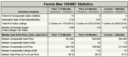
Figure 1 shows changes in this sub-market over time

At this point, the analysis will compare the median comparable sales price from 7-12 months ago to that of 4-6 months ago.  Note this will be a positive change since, across those time periods, the sales price increased.  Figure 2 shows the key strokes, as well as the change in value.

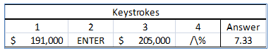
Figure 2 shows the keystrokes

What Figure 2 makes clear is that, in the eight (8) months from 12-months ago to 4-months ago, priced increased 7.33%, or an average of 0.92% (0.0092) per month.  Say a property sold for $100,000 five (5) months ago.  To make the adjustment, then, first multiply the change factor (0.0092) times five (5) months to arrive at the total factor (0.0092 X 5 =) 0.0460.  Now add one (1) [this does not mean 1-cubed.  It means see footnote #3] to the factor.  Do this by touching the “enter” key, then the numeral one, then the “plus” (+) sign.  The display window will show “1.0460.”  Now press the “enter” key, then 100000, then the “X” (multiply) key. This multiplies the change factor by the original purchase price to arrive at the purchase price modified by the change in value factor over time.  The display window will show “104600,” or $104,600 to be the “time-adjusted” purchase price.

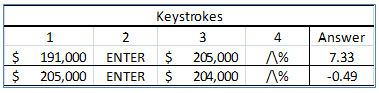
Figure 3 shows the 2nd Price Change over Time; this time the change is negative

Now consider Figure 3. It shows that from yesterday, going back six months, prices fell by a factor of 0.0049 (that’s 0.49%), or a monthly average factor of 0.000817 per month. In reality, this decrease is so slight, that it would be proper to call the market stable, thus not adjust a sale from one month ago. To go through the math, though, would be to multiply the purchase price (here a hypothetical $100,000) by the factor 0.000817 (the factor for one month), to arrive at a decrease in value of $81.70. Now, deduct this from the sales price to arrive at an adjusted price of $99,918. Since markets are not this precise, to actually make this adjustment could be construed as misleading, a violation of USPAP SR2-1(a), in that such a step might delude the client and/or intended user to conclude the appraiser actually knew the value of a property to the nearest one dollar. This level of precision is simply not true, so there is no reason to imply it.

(story continues below)

(story continues)

So what is the interpretation of this negative price change in the recent past? Given that the longer trend (i.e., from $191,000 to $204,000) is up annually at 6.8%, the trend over time is still increasing. However, what these data show is that the trend line, instead of continuing to increase, has leveled out; indeed, it may be trending downward very slowly. However, there are not enough data yet to determine if the long-term trend is indeed downward or this is merely a seasonal (or one-time) glitch with no real meaning or impact on value. To explain this to the client, the appraiser could consider something such as the language in this paragraph:

“From these recent sales data, two trends are evident. First, that values are up over time is clear. The evidence is that median sales prices increased to $204,000 from $191,000 over the last 12-months. Despite this overall trend, the most recent price change was ever-so-slightly downward. Median sales price decreased to $204,000 from $205,000. This change, in and of itself, is minor and is likely due to nothing more important than natural market cycles. However, it bears watching over time. Given this dynamic, as well as the fact that all of the comparables went under contract in the last six (6) months, and closed escrow within the last four (4) months, the appraiser concluded no time adjustment, either up or down, was necessary for the comparable sales and listings herein.”

There are other ways to calculate a “time” adjustment. However, this process is likely the most direct, quickest, as well as the most subject-specific. Just because prices went up over time in an entire MSA (metropolitan statistical area), does not mean that prices went up at that same rate (or at all!) in one of the MSA’s sub-markets.

As the introduction indicated, an analysis of this type is basically paired sales analysis. However, instead of pairing individual sales of individual properties, this is a pairing of the median values of many sales over time. Frankly, there is no one best way to calculate a time adjustment. This one, while approximate at best, relies on an obvious change in median prices over three distinct time intervals. There is likely less observational bias in this method than there is in trying to draw a time adjustment from just five or six sales over a single long interval. Therefore, while the introduction mentioned three ways to calculate a time adjustment, an explanation of this one method suffices.

It is not necessary to include details of a process this complex and detailed in a residential appraisal report (especially if it is for typical FNMA mortgage lending purposes). A precise summary of the data and their analyses will suffice. However, keep all of this in the work file for future reference. To keep all of these data and analyses in a workfile is to be well prepared if the state or a plaintiff ever comes calling!

New Online CE – 7 Hours
How To Support and Prove Your Adjustments
Presented by: Richard Hagar, SRA

Do you have the proper support for your adjustments? Stop taking the same old CE courses and learn proven adjustment methods with instructor Richard Hagar, SRA. Fannie Mae states that the number one reason appraisals are flagged is the “use of adjustments that do not reflect market reaction.” Stay out of trouble with Fannie Mae, your state board and your AMC/lender clients with solid, supportable adjustments.  Up your game, avoid time-consuming callbacks and earn approved CE today!

“Why wasn’t this taught years ago?” – Jackie Henry

How to Support and Prove Your Adjustments
Sign Up Now!  $119  – 7 Hrs. Approved CE
(OREP Member Price: $99)

About the Author
Timothy C. Andersen, MAI is the author of the Expert’s Guide to a Defensible Workfile and has been in real estate and consulting since 1975. He is a commercial real estate appraiser, AQB-certified USPAP instructor, USPAP consultant, Special Magistrate for the Palm Beach County Value Adjustment Board, author, instructor and expert witness. As a USPAP consultant, he works nationwide as an expert with appraisers whom the state has charged with license law violations. He is an instructor with the Appraisal Institute and has worked all over the U.S. with various proprietary schools, as well as a community college. The University of St. Thomas in Minneapolis, MN recently awarded him a Master of Science degree in Real Estate Appraisal. Tim’s e-mail address is maitca@bellsouth.net.

> Click to Print

Send your story submission/idea to the Editor: isaac@orep.org